Numerical Codes

A collection of numerical software for studying nonlinear waves, quantum fluids, and two-dimensional turbulence from continuous fields resolved in Fourier space to interacting systems of discrete vortices.

Each code is written in modern C++ and includes reproducible examples, diagnostics, restart support, and plotting and movie scripts. The repositories contain full installation and usage guides.

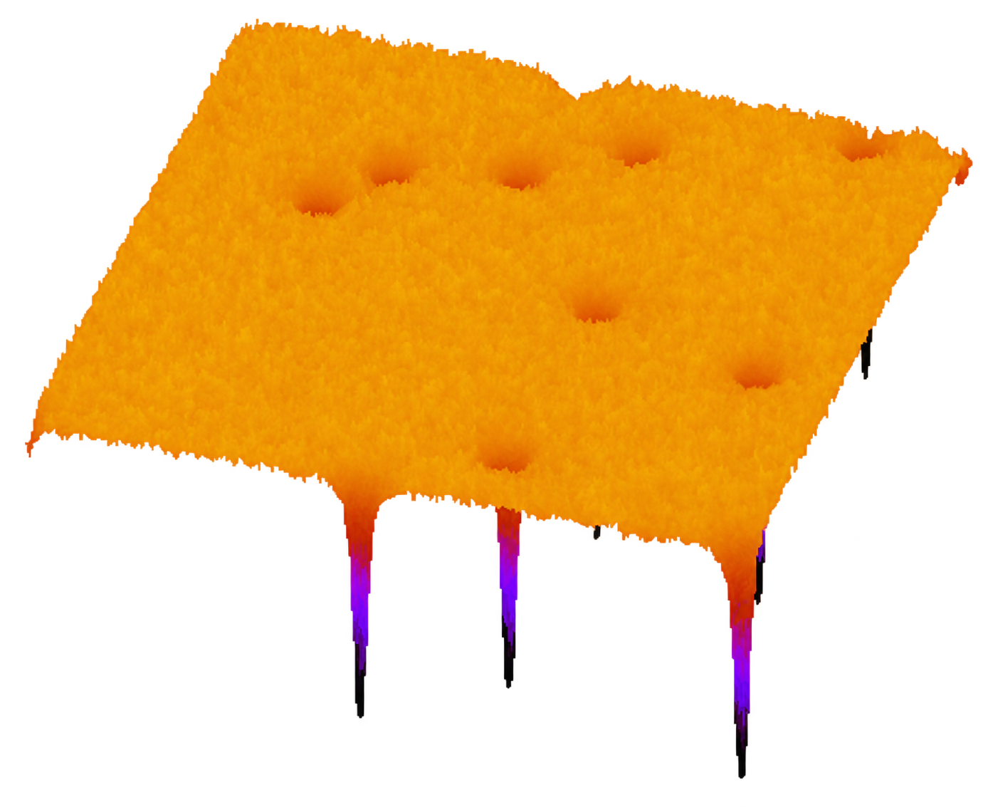
Isolated soliton field from the one-dimensional Schrödinger–Helmholtz model — Relaxation of a nonlinear Schrödinger soliton into a soliton bound state in the one-dimensional Schrödinger–Helmholtz model.

Nonlinear optical waves

1D Schrödinger–Helmholtz

A pseudo-spectral solver for the nonlocal 1D Schrödinger–Helmholtz equation and two closely related limits. It is designed to explore nonlocal optical wave turbulence, coherent structures, and the transition from nonlocal to local nonlinear dynamics on a periodic one-dimensional domain.

Governing equation

i∂_tψ = c∂_xxψ+ gψ(1 − β∂_xx)⁻¹|ψ|²+ μψ

Here ψ(x,t) is a complex wave field and the inverse Helmholtz operator smooths the nonlinear density response over a scale set by β. Configurable forcing and large- and small-scale damping may also be included.

A single model setting also selects the long-wave approximation (1 + β∂_xx)|ψ|² or the local cubic nonlinear Schrödinger equation. All variants use a fully dealiased pseudo-spectral nonlinear evaluation and fixed-step exponential or integrating-factor time integrators.

Three optical wave models
Stochastic or single-mode forcing
FFTW and optional OpenMP

View the GitHub repository

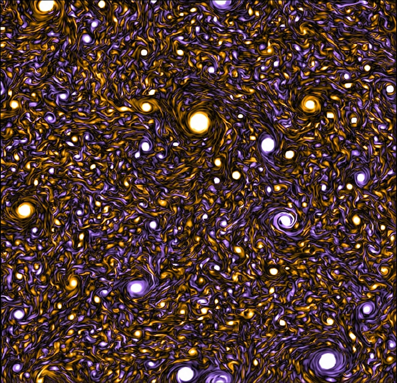
Gross–Pitaevskii density field containing several quantised vortices — Gross–Pitaevskii density field showing Bogoliubov waves and quantised vortices.

Quantum fluids

2D Gross–Pitaevskii

A parallel pseudo-spectral solver for a complex 2D Gross–Pitaevskii equation on a doubly periodic domain. The model describes weakly interacting Bose gases and superfluids, as well as 2D nonlinear optical propagation defined through a Kerr nonlniearity. The model resolves both dispersive waves and quantised vortices within a single field equation.

Conservative governing equation

i∂_tψ = c∆ψ+ g|ψ|²ψ + μψ

The complex field ψ(x,t) contains the fluid density |ψ|² and phase. Optional Ginzburg–Landau damping, spectral dissipation, and external forcing extend the equation to driven, non-equilibrium systems.

The cubic nonlinearity is evaluated with a two-pass 3/2 dealiasing rule. CPU/OpenMP, hybrid MPI/OpenMP, and NVIDIA CUDA executables share the same model, inputs, output, and checkpoint format, making it possible to move a calculation between platforms.

Focussing/defocussing nonlinearity
Fully dealiased
CPU, MPI, and CUDA backends

View the GitHub repository

Complex vortical structures in a two-dimensional turbulent flow — Vorticity field of a two-dimensional Navier–Stokes turbulent flow.

Classical turbulence

2D Navier–Stokes

A parallel pseudo-spectral solver for incompressible 2D Navier-Stokes flow in vorticity form. It supports forced and decaying turbulence, ordinary or scale-selective dissipation, and an optional beta-plane term for idealised geophysical flows.

Governing equation

∂_tω + u · ∇ω + β∂_xψ= −ν(−∆)^pω− α(−∆)^qω + F

ω = ∆ψ,u = (−∂_yψ, ∂_xψ)

The vorticity ω determines the streamfunction ψ and incompressible velocity u. The coefficients ν and α control small- and large-scale dissipation, while F injects vorticity into selected Fourier modes.

Nonlinear advection is evaluated on a fully padded 3/2-rule grid. The solver records energy and enstrophy, their spectra and fluxes, and runs through matching CPU/OpenMP, hybrid MPI/OpenMP, and NVIDIA CUDA implementations.

Beta-plane dynamics
Energy and enstrophy diagnostics
CPU, MPI, and CUDA backends

View the GitHub repository

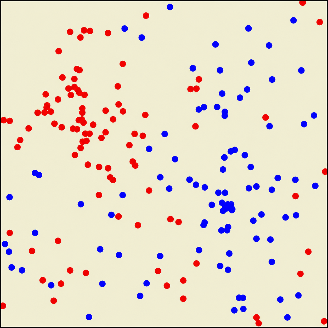
Positive and negative point vortices distributed across a periodic domain — A turbulent point-vortex flow displaying clustering of same-signed vortices.

Vortex dynamics

2D point vortices

A direct N-body solver for two-dimensional point-vortex dynamics. Instead of resolving a continuous velocity field, it follows idealised vortices with fixed circulations as they advect one another through the Biot–Savart interaction.

Equations of motion in the infinite plane

dx_idt= −12π∑_j≠i Γ_jy_i−y_jr_ij²+ε²dy_idt= 12π∑_j≠i Γ_jx_i−x_jr_ij²+ε²

Vortex i has position (x_i, y_i) and circulation Γ_i; ε optionally regularises close encounters. Geometry-specific kernels provide singly periodic, doubly periodic, and circular-disk domains as well as the infinite plane shown here.

The solver uses direct all-pairs velocity sums with adaptive Dormand–Prince time integration. CPU/OpenMP, MPI, and CUDA backends use identical input, trajectory, diagnostics, and checkpoint formats. The solver includes bespoke forcing and dissipation algorithms to study out-of-equilibrium point vortex motion.

Four domain geometries
Adaptive timestepping
CPU, MPI, and CUDA backends

View the GitHub repository